The Grey Level Cooccurence Matrix (GLCM) has been described in the
image processing literature by a number of names including Spatial
Grey Level Dependence (SGLD) [CH80] etc. As the
name suggests, the GLCM is constructed from the image by estimating
the pairwise statistics of pixel intensity. Each element (i,j) of
the matrix represents an estimate of the probability that two pixels
with a specified separation have grey levels i and j. The
separation is usually specified by a displacement, d and an angle,
![]() . That is,
. That is,
![]()
![]() will be a square matrix of side equal to
the number of grey levels in the image and will usually not be
symmetric. Symmetry is often introduced by effectively adding the
GLCM to it's transpose and dividing every element by 2. This renders
will be a square matrix of side equal to
the number of grey levels in the image and will usually not be
symmetric. Symmetry is often introduced by effectively adding the
GLCM to it's transpose and dividing every element by 2. This renders
![]() and
and ![]() identical and
makes the GLCM unable to detect
identical and
makes the GLCM unable to detect ![]() rotations.
rotations.
In texture classification, individual elements of the GLCM are rarely
used. Instead, features are derived from the matrix. A large number
of textural features have been proposed starting with the original
fourteen features described by Haralick et al [HSD73],
however only some of these are in wide use. Wezska et al
[WDR76] used four of Haralick et al's fourteen features
( ![]() ,
, ![]() ,
, ![]() ,
, ![]() ). Conners and Harlow [CH80]
use five features (
). Conners and Harlow [CH80]
use five features ( ![]() ,
, ![]() ,
, ![]() ,
, ![]() ,
, ![]() ). Conners,
Trivedi and Harlow [CTH84] introduced two new features
which address a deficiency in the Conners and Harlow set (
). Conners,
Trivedi and Harlow [CTH84] introduced two new features
which address a deficiency in the Conners and Harlow set ( ![]() ,
,
![]() ,
, ![]() ,
, ![]() ,
, ![]() ,
, ![]() ). The features listed above are
defined as
). The features listed above are
defined as
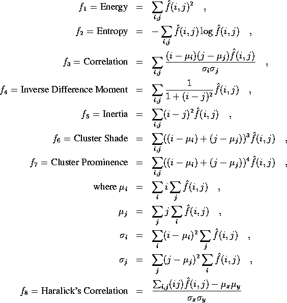
where ![]() ,
, ![]() ,
, ![]() and
and ![]() are the means and
standard deviations of row and column sums, respectively.
are the means and
standard deviations of row and column sums, respectively.
For any choice of d and ![]() we obtain a separate GLCM,
generally sensitive to the value of d and
we obtain a separate GLCM,
generally sensitive to the value of d and ![]() . The GLCM is
commonly implemented with some degree of rotation invariance. This is
usually achieved by combining the results of a subset of angles. If
the GLCM is calculated with symmetry, then only angles up to
. The GLCM is
commonly implemented with some degree of rotation invariance. This is
usually achieved by combining the results of a subset of angles. If
the GLCM is calculated with symmetry, then only angles up to
![]() need be considered and the four angles
need be considered and the four angles ![]() are an effective choice. The results
may be combined by averaging the GLCM for each angle before
calculating the features or by averaging the features calculated for
each GLCM. Separate feature sets are now obtainable for different
values of d, irrespective of
are an effective choice. The results
may be combined by averaging the GLCM for each angle before
calculating the features or by averaging the features calculated for
each GLCM. Separate feature sets are now obtainable for different
values of d, irrespective of ![]() , however, values other than 1
are rarely used.
, however, values other than 1
are rarely used.
This algorithm has been implemented in the program glcmClass.
The Gabor Energy method measures the similarity between neighbourhoods
in an image and Gabor masks. Each Gabor mask consists of Gaussian
windowed sinusoidal waveforms. Masks can be generated for varying
wavelength ( ![]() ), orientation (
), orientation ( ![]() ), phase shift (
), phase shift ( ![]() ),
and Gaussian window standard deviation (
),
and Gaussian window standard deviation ( ![]() ) using
) using
![]()
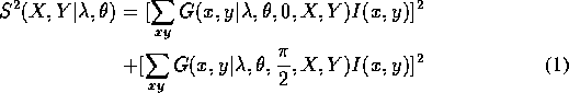
The energy is computed at each pixel for each combination of wavelength and orientation ; the energy is the sum, over the phases, of the squared convolution values. That is, if we let the image be I(x,y), then
Energy calculated using equation 1 for
each combination of ![]() and
and ![]() may be used as texture
features [FS89].
may be used as texture
features [FS89].
A Gabor mask is a sinusoidal waveform which is spatially localised by modulation with a Gaussian envelope. Mathematically, the family of Gabor convolutions is a spatially localised modification of a Fourier analysis. Fourier analyses describe waveforms ; specifically the frequency and orientation of waveforms. Most authors motivate the use of Gabor convolutions by relating them to Fourier analyses.
Another point of view regards the Gabor masks as texton detectors. Textons are spatially local patterns such as oriented lines, line ends, edges and blobs. According to the texton theory of human texture discrimination, preattentive human texture discrimination can be modeled by the first order density of textons and second order statistics of intensity.
So far, we have described the distinction between the Fourier and Texton approaches to Gabor convolutions at a theoretical level. At a practical level, the Fourier and Texton approaches are distinguished by the ratio between the wavelength of the sinusoid and the width of the Gaussian envelope in a Gabor mask. If the Gaussian envelope is large enough to contain several wavelengths, then the Gabor mask will be sensitive to the orientation of the waveform peaks, the width of the peaks and the interpeak distance. In brief, such a Wide mask will detect features appropriate to a Fourier analysis. However, if the Gaussian envelope is approximately one wavelength in width, the Gabor mask will be sensitive to the orientation and width of the peaks, but not the interpeak distance. In brief, such a Narrow mask will detect features appropriate to measuring texton density.
Figure 1 gives examples of both Wide and Narrow masks.
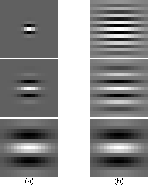
Figure 1: Gabor Convolution Masks for wavelengths of 2, 4 and 8 pixels with (a) Narrow envelope and (b) Wide envelope.
This algorithm has been implemented in the program gaborClass.
Gaussian Markov Random Field (GMRF) methods characterise the statistical relationship between a pixel and its neighbours [CC85]. A stochastic model results where the number of parameters is equal to the size of the neighborhood mask. The parameters are calculated using a LMS algorithm over every valid mask position in the image. A commonly used mask is the symmetric fourth-order mask shown in Figure 2.
Consider a zero mean image, I(s) [s=(i,j)] and assume the pixel values
are Gaussian. Let the neighbourhood be defined by the set ![]() where each element is a pixel location relative to the
current pixel i.e. (0,1) indicates image pixel I(i,j+1). Now, assume
that the pixels in the image are related by
where each element is a pixel location relative to the
current pixel i.e. (0,1) indicates image pixel I(i,j+1). Now, assume
that the pixels in the image are related by
Using a symmetric mask and allowing a ![]() rotation invariance,
the number of parameters can be halved, as the parameters are made
common between I(s+r) and I(s-r) as in
rotation invariance,
the number of parameters can be halved, as the parameters are made
common between I(s+r) and I(s-r) as in
The model parameters are obtained by solving for ![]() in
equations 2 or 3 using a Least Squares
method detailed by Chellappa and Chatterjee
[CC85].
in
equations 2 or 3 using a Least Squares
method detailed by Chellappa and Chatterjee
[CC85].
Figure 2: GMRF fourth-order mask.
This algorithm has been implemented in the program markovClass.
The use of Fractal Dimension (FD) for texture classification and segmentation has been proposed by a number of researchers [CSK93, KC89, Pen84, PNHA84]. The property of self-similarity implies that the FD of an image will be independent of scale. This phenomenum was observed by Pentland [Pen84].
Various methods exist to estimate the FD of an image ; 2D generalization of Mandelbrot's original methods for coastlines [PNHA84], Fourier-transform based methods [Pen84], and variations on box-counting [KC89, CSK93].
The principle of self-similarity may be stated as: If a bounded
set A is composed of ![]() non-overlapping copies of a set similar
to A, but scaled down by a factor r, then A is self-similar.
From this definition, the FD is given by
non-overlapping copies of a set similar
to A, but scaled down by a factor r, then A is self-similar.
From this definition, the FD is given by
![]()
FD can
be approximated by estimating ![]() for various values of r and then
determining the slope of the least-squares linear fit of
for various values of r and then
determining the slope of the least-squares linear fit of ![]() Vs
Vs
![]() . The differential box-counting method outlined in
Chaudhuri et al [CSK93] may be used to achieve this
task.
. The differential box-counting method outlined in
Chaudhuri et al [CSK93] may be used to achieve this
task.
Consider an ![]() pixel image as a surface in (x,y,z)
space where (x,y) represents the pixel position and z is the
pixel intensity. We now partition the (x,y) space into a grid of
size
pixel image as a surface in (x,y,z)
space where (x,y) represents the pixel position and z is the
pixel intensity. We now partition the (x,y) space into a grid of
size ![]() pixels. An estimate of the relative scale is
pixels. An estimate of the relative scale is ![]() . At each grid position, we stack cubes of size s,
numbering each box sequentially from 1 up to the box containing the
highest intensity in the image over the
. At each grid position, we stack cubes of size s,
numbering each box sequentially from 1 up to the box containing the
highest intensity in the image over the ![]() area.
area.
Denoting the boxes containing the minimum and maximum grey levels for
the image in the ![]() area at grid position (i,j) by k and
l respectively, we define
area at grid position (i,j) by k and
l respectively, we define ![]() . This is the
differential variation of the box-counting method.
. This is the
differential variation of the box-counting method. ![]() is estimated
by summing over the entire grid as
is estimated
by summing over the entire grid as ![]() .
.
The above procedure is repeated for a number of values of r (s)
and ![]() versus
versus ![]() is plotted. FD is then estimated by
the gradient of the least-squares linear fit of these points.
is plotted. FD is then estimated by
the gradient of the least-squares linear fit of these points.
To compensate for "image regularity", two random shifts of the box columns are introduced. The first purturbates the grid position of the column while the second introduces a random offset into the column height of less than one full box height.
Four features are extracted as per Chaudhuri et al [CSK93]. They are
![]()
where ![]() , and
, and ![]() and
and ![]() are the minimum and average grey values in
are the minimum and average grey values in ![]() .
.
![]()
where ![]() , and
, and ![]() and
and ![]() are the maximum and average grey values in
are the maximum and average grey values in ![]() .
.
The first three features are calculated as above on the appropriately
modified images. The fourth feature is based on multifractals which
are used for self-similar distributions exhibiting non-isotropic and
inhomogeneous scaling properties. Using the notation as before, we
introduce ![]() . The multifractal FD, D(2) is
then
. The multifractal FD, D(2) is
then
![]()
A number of different values for r are used and the linear
regression of ![]() versus
versus ![]() yields an
estimate D(2).
yields an
estimate D(2).
All features are normalized to lie between 0.0 and 1.0.
This algorithm has been implemented in the program fractalClass.